Solving XOR with a Neural Network in TensorFlow

The tradition of writing a trilogy in five parts has a long and noble history, pioneered by the great Douglas Adams in the Hitchhiker’s Guide to the Galaxy. This post is no exception and follows from the previous four looking at a Neural Network that solves the XOR problem.

This time, I had a interest in checking out Google’s machine learning system, TensorFlow.

Last November, Google open sourced the machine learning library that it uses within their own products. There are two API’s; one for Python and one for C++.  Naturally, it makes sense to see what TensorFlow would make of the same network that we previously looked at and compare both Python-based neural networks.

You can download the TensorFlow library and see some of the tutorials here.

It’s worth noting that TensorFlow requires a little mental agility to understand. Essentially. the first few lines of code set up the inputs, the network architecture, the cost function, and the method to use to train the network. Although these look like the same steps as the steps in Python or Octave, they don’t in fact do anything. This is because TensorFlow considers those to be the model to use, running them only within a session. This model is in the form of a directed graph. Don’t worry if that’s not too clear yet.

TensorFlow Code

To start with, we need to load in the TensorFlow library:

import tensorflow as tf

The next step is to set up placeholders to hold the input data. TensorFlow will automatically fill them with the data when we run the network. In our XOR problem, we have four different training examples and each example has two features. There are also four expected outputs, each with just one value (either a 0 or 1). In TensorFlow, this looks like this:

x_ = tf.placeholder(tf.float32, shape=[4,2], name="x-input")
y_ = tf.placeholder(tf.float32, shape=[4,1], name="y-input")

I’ve set up the inputs to be floating point numbers rather than the more natural integers to avoid having to cast them to floating points when multiplying the weights later on. The shape parameter tells the placeholder what the dimensions are of data we’ll be passing in.

The next step is to set up the parameters for the network. These are called Variables in TensorFlow.  Variables will be modified by TensorFlow during the training steps.

Theta1 = tf.Variable(tf.random_uniform([2,2], -1, 1), name="Theta1")
Theta2 = tf.Variable(tf.random_uniform([2,1], -1, 1), name="Theta2")

For our Theta matrices, we want them initialized to random values between -1 and +1, so we use the built-in random_uniform function to do that.

In TensorFlow, we set up the bias nodes separately, but still as Variables. This let’s the algorithms modify the values of the bias node. This is mathematically equivalent to having a signal value of 1 and initial weights of 0 on the links from the bias nodes.

Bias1 = tf.Variable(tf.zeros([2]), name="Bias1")
Bias2 = tf.Variable(tf.zeros([1]), name="Bias2")

Now we set up the model. This is pretty much the same as that outlined in the previous posts on Python and Octave:

A2 = tf.sigmoid(tf.matmul(x_, Theta1) + Bias1)
Hypothesis = tf.sigmoid(tf.matmul(A2, Theta2) + Bias2)

Here, matmul is TensorFlow’s matrix multiplication function, and sigmoid naturally is the sigmoid calculation function.

As before, our cost function is the average over all the training examples:

cost = tf.reduce_mean(( (y_ * tf.log(Hypothesis)) + 
        ((1 - y_) * tf.log(1.0 - Hypothesis)) ) * -1)

So far, that has been relatively straightforward. Let’s look at training the network.

TensorFlow ships with several different training algorithms, but for comparison purposes with our previous implementations, we’re going to use the gradient descent algorithm:

train_step = tf.train.GradientDescentOptimizer(0.01).minimize(cost)

What this statement says is that we’re going to use GradientDescentOptimizer as our training algorithm, the learning rate (alpha from before) is going to be 0.01 and we want to minimize the cost function above. This means that we don’t have to implement our own algorithm as we did in the previous examples.

That’s all there is to setting up the network. Now we just have to go through a few initialization steps before running the examples through the network:

XOR_X = [[0,0],[0,1],[1,0],[1,1]]
XOR_Y = [[0],[1],[1],[0]]

init = tf.global_variables_initializer()
sess = tf.Session()
sess.run(init)

As I mentioned above, TensorFlow runs a model inside a session, which it uses to maintain the state of the variables as they are passed through the network we’ve set up. So the first step in that session is to initialise all the Variables from above. This step allocates values to the various Variables in accordance with how we set them up (i.e. random numbers for Theta and zeros for Bias).

The next step is to run some epochs:

for i in range(100000):
        sess.run(train_step, feed_dict={x_: XOR_X, y_: XOR_Y})

Each time the training step is executed, the values in the dictionary feed_dict are loaded into the placeholders that we set up at the beginning. As the XOR problem is relatively simple, each epoch will contain the entire training set. To see what’s going on inside the loop, just print out the values of the Variables:

if i % 1000 == 0:
        print('Epoch ', i)
        print('Hypothesis ', sess.run(Hypothesis, feed_dict={x_: XOR_X, y_: XOR_Y}))
        print('Theta1 ', sess.run(Theta1))
        print('Bias1 ', sess.run(Bias1))
        print('Theta2 ', sess.run(Theta2))
        print('Bias2 ', sess.run(Bias2))
        print('cost ', sess.run(cost, feed_dict={x_: XOR_X, y_: XOR_Y}))

That’s it. If you run this in Python, you’ll get something that looks like this after 99000 epochs:

As you can see in the display for the Hypothesis variable, the network has learned to output nearly correct values for the inputs.

 

The TensorFlow Graph

I mentioned above that the model was in the form of a directed graph. TensorFlow let’s us see what that graph looks like:

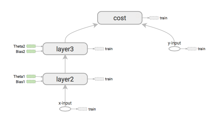
We can see that our inputs x-input and y-input are the starts of the graph, and that they flow through the processes at layer2 and layer3, ultimately being used in the cost function.

To see the graph yourself, TensorFlow includes a utility called TensorBoard. Inside your code, before the sess.run(init) statement add the following line:

writer = tf.summary.FileWriter("./logs/xor_logs", sess.graph_def)

The folder in the quotes can point to a folder on your machine where you want to store the output. Running TensorBoard is then as simple as entering this at a command prompt:

$ tensorboard --logdir=/path/to/your/log/file/folder

In your browser, enter http://localhost:6006 as the URL and then click on Graph tab. You will then see the full graph.

So that’s an example neural network in TensorFlow.

There is one thing I did notice in putting this together: it’s quite slow. In Octave, I was able to run 10,000 epochs in about 9.5 seconds. The Python/NumPy example was able to run in 5.8 seconds. The above TensorFlow example runs in about 28 seconds on my laptop.

TensorFlow is however built to run on GPUs and the model can be split across multiple machines. This would go some way to improving performance, but there is a way to go to make it comparable with existing libraries.

UPDATE 26/01/2016:

I’ve placed the full code up on GitHub here: https://github.com/StephenOman/TensorFlowExamples/tree/master/xor%20nn

Enjoy!

Update 07/03/2016:

I’ve changed the GitHub code to run a more realistic 100,000 epochs. Should converge now. [Thanks Konstantin!]