XOR Revisited: Keras and TensorFlow

A few weeks ago, it was announced that Keras would be getting official Google support and would become part of the TensorFlow machine learning library. Keras is a collection of high-level APIs in Python for creating and training neural networks, using either Theano or TensorFlow as the underlying engine.

Given my previous posts on implementing an XOR-solving neural network in a variety of different languages and tools, I thought it was time to see what it would look like in Keras.

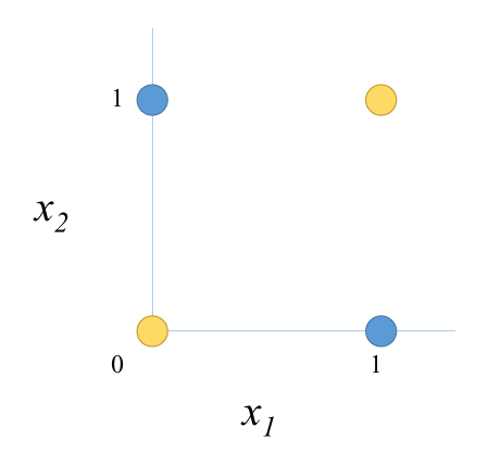
XOR can be expressed as a classification problem that is best illustrated in a diagram. The goal is to create a neural network that will correctly predict the values 0 or 1, depending on the inputs x1 and x2 as shown.

The neural network that is capable of being trained to solve that problem looks like this:

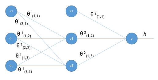
If you’d like to understand why this is the case, have a look at the detailed explanation in the posts implementing the solution in Octave.

So how does this look in Keras? Well it’s rather simple. Assuming you’ve already installed Keras, we’ll start with setting up the classification problem and the expected outputs:

import numpy as np

x = np.array([[0,0], [0,1], [1,0], [1,1]])
y = np.array([[0], [1], [1], [0]])

So far, so good. We’re using numpy arrays to store our inputs (x) and outputs (y). Now for the neural network definition:

from keras.models import Sequential
from keras.layers import Dense, Activation

model = Sequential()
model.add(Dense(2, input_shape=(2,)))
model.add(Activation('sigmoid'))
model.add(Dense(1))
model.add(Activation('sigmoid'))

The Sequential model is simply a sequence of layers making up the network. Our diagram above has a set of inputs being fed into two processing layers. We’ve already defined the inputs, so all we need to do is add the other two layers.

In Keras, we’ll use Dense layers, which simply means they are is fully connected. The parameters indicate that the first layer has two nodes and the second layer has one node, corresponding to the diagram above.

The first layer also has the shape of the inputs which in this case is a one-dimensional vector with 2 elements. The second layer’s inputs will be inferred from the first layer.

We then add an Activation of type ‘sigmoid’ to each layer, again matching our neural network definition.

Note that Keras looks after the bias input without us having to explicitly code for it. In addition, Keras also looks after the weights (Θ1 and Θ2). This makes our neural network definition really straightforward and shows the benefits of using a high-level abstraction.

Finally, we apply a loss function and learning mode for Keras to be able to adjust the neural network:

model.compile(loss='mean_squared_error', optimizer='sgd', metrics=['accuracy'])

In this example, we’ll use the standard Mean Squared Error loss function and Stochastic Gradient Descent optimiser. And that’s it for the network definition.

If you want to see that the network looks like, use:

model.summary()

The network should look like this:

>> model.summary()
_________________________________________________________________
Layer (type)                  Output Shape         Param # 
=================================================================
dense_1 (Dense)               (None, 2)            6 
_________________________________________________________________
activation_1 (Activation)     (None, 2)            0 
_________________________________________________________________
dense_2 (Dense)               (None, 1)            3 
_________________________________________________________________
activation_2 (Activation)     (None, 1)            0 
=================================================================
Total params: 9
Trainable params: 9
Non-trainable params: 0
_________________________________________________________________
>>>

Now we just need to kick off the training of the network.

model.fit(x,y, epochs=100000, batch_size=4)

All going well, the network weights will converge on a solution that can correctly classify the inputs (if not, you may need to up the number of epochs):

>>> model.predict(x, verbose=1)

4/4 [==============================] - 0s

array([[ 0.07856689],

       [ 0.91362464],

       [ 0.92543262],

       [ 0.06886736]], dtype=float32)

>>>

Clearly this network is on it’s way to converging on the original expected outputs we defined above (y).

So that’s all there is to a Keras version of the XOR-solving neural network. The fact that it is using TensorFlow as the engine is completely hidden and that makes implementing the network a lot simpler.