Introduction
This post demonstrates the calculations behind the evaluation of the Softmax Derivative using Python. It is based on the excellent article by Eli Bendersky which can be found here.
The Softmax Function
The softmax function simply takes a vector of N dimensions and returns a probability distribution also of N dimensions. Each element of the output is in the range (0,1) and the sum of the elements of N is 1.0.
Each element of the output is given by the formula:

See https://en.wikipedia.org/wiki/Softmax_function for more details.
import numpy as np
x = np.random.random([5])

def softmax_basic(z):
    exps = np.exp(z)
    sums = np.sum(exps)
    return np.divide(exps, sums)

softmax_basic(x)
This should generate an output that looks something like this:
array([0.97337094, 0.85251098, 0.62495691, 0.63957056, 0.6969253 ])
We expect that the sum of those will be (close to) 1.0:
np.sum(softmax_basic(x))
And so it is:
1.0
Calculating the derivative
We need to calculate the partial derivative of the probability outputs 


Following Bendersky’s derivation, we need to use the quotient rule for derivatives:
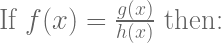
![f'(x)=\frac{g'(x)h(x)-h'(x)g(x)}{[h(x)]^{2}}](https://s0.wp.com/latex.php?latex=f%27%28x%29%3D%5Cfrac%7Bg%27%28x%29h%28x%29-h%27%28x%29g%28x%29%7D%7B%5Bh%28x%29%5D%5E%7B2%7D%7D&bg=ffffff&fg=5e5e5e&s=3&c=20201002)
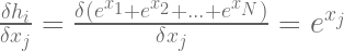
From the Softmax function:

The derivatives of these functions with respect to

and
Now we have to evalutate the quotient rule for the two seperate cases where 

Starting with
![\frac{\delta{\frac{e^{x_{i}}} {\sum_{k=1}^N e^{x_{k}}}}}{\delta{x_{j}}}=\frac{e^{x_{j}}\sum_{k=1}^N e^{x_{k}}-e^{x_{j}}e^{x_{i}}}{\left[\sum_{k=1}^N e^{x_{k}}\right]^{2}}](https://s0.wp.com/latex.php?latex=%5Cfrac%7B%5Cdelta%7B%5Cfrac%7Be%5E%7Bx_%7Bi%7D%7D%7D+%7B%5Csum_%7Bk%3D1%7D%5EN+e%5E%7Bx_%7Bk%7D%7D%7D%7D%7D%7B%5Cdelta%7Bx_%7Bj%7D%7D%7D%3D%5Cfrac%7Be%5E%7Bx_%7Bj%7D%7D%5Csum_%7Bk%3D1%7D%5EN+e%5E%7Bx_%7Bk%7D%7D-e%5E%7Bx_%7Bj%7D%7De%5E%7Bx_%7Bi%7D%7D%7D%7B%5Cleft%5B%5Csum_%7Bk%3D1%7D%5EN+e%5E%7Bx_%7Bk%7D%7D%5Cright%5D%5E%7B2%7D%7D+&bg=ffffff&fg=5e5e5e&s=3&c=20201002)
Now we’ll just simplify this a bit:
![\begin{array}{rcl} \frac{\delta{\frac{e^{x_{i}}} {\sum_{k=1}^N e^{x_{k}}}}}{\delta{x_{j}}} & = & \frac{e^{x_{j}}\left(\sum_{k=1}^N e^{x_{k}}-e^{x_{i}}\right)}{\left[\sum_{k=1}^N e^{x_{k}}\right]^{2}}\\ &=&\frac{e^{x_{j}}}{\sum_{k=1}^N e^{x_{k}}} \dot{}\frac{\sum_{k=1}^N e^{x_{k}}-e^{x_{i}}}{\sum_{k=1}^N e^{x_{k}}}\\ &=&\frac{e^{x_{j}}}{\sum_{k=1}^N e^{x_{k}}} \left(\frac{\sum_{k=1}^N e^{x_{k}}}{\sum_{k=1}^N e^{x_{k}}}-\frac{e^{x_{i}}}{\sum_{k=1}^N e^{x_{k}}}\right)\\ &=&\frac{e^{x_{j}}}{\sum_{k=1}^N e^{x_{k}}} \left(1-\frac{e^{x_{i}}}{\sum_{k=1}^N e^{x_{k}}}\right)\\ &=&\sigma(x_{j})(1-\sigma(x_{i})) \end{array}](https://s0.wp.com/latex.php?latex=%5Cbegin%7Barray%7D%7Brcl%7D+%5Cfrac%7B%5Cdelta%7B%5Cfrac%7Be%5E%7Bx_%7Bi%7D%7D%7D+%7B%5Csum_%7Bk%3D1%7D%5EN+e%5E%7Bx_%7Bk%7D%7D%7D%7D%7D%7B%5Cdelta%7Bx_%7Bj%7D%7D%7D+%26+%3D+%26+%5Cfrac%7Be%5E%7Bx_%7Bj%7D%7D%5Cleft%28%5Csum_%7Bk%3D1%7D%5EN+e%5E%7Bx_%7Bk%7D%7D-e%5E%7Bx_%7Bi%7D%7D%5Cright%29%7D%7B%5Cleft%5B%5Csum_%7Bk%3D1%7D%5EN+e%5E%7Bx_%7Bk%7D%7D%5Cright%5D%5E%7B2%7D%7D%5C%5C+%26%3D%26%5Cfrac%7Be%5E%7Bx_%7Bj%7D%7D%7D%7B%5Csum_%7Bk%3D1%7D%5EN+e%5E%7Bx_%7Bk%7D%7D%7D+%5Cdot%7B%7D%5Cfrac%7B%5Csum_%7Bk%3D1%7D%5EN+e%5E%7Bx_%7Bk%7D%7D-e%5E%7Bx_%7Bi%7D%7D%7D%7B%5Csum_%7Bk%3D1%7D%5EN+e%5E%7Bx_%7Bk%7D%7D%7D%5C%5C+%26%3D%26%5Cfrac%7Be%5E%7Bx_%7Bj%7D%7D%7D%7B%5Csum_%7Bk%3D1%7D%5EN+e%5E%7Bx_%7Bk%7D%7D%7D+%5Cleft%28%5Cfrac%7B%5Csum_%7Bk%3D1%7D%5EN+e%5E%7Bx_%7Bk%7D%7D%7D%7B%5Csum_%7Bk%3D1%7D%5EN+e%5E%7Bx_%7Bk%7D%7D%7D-%5Cfrac%7Be%5E%7Bx_%7Bi%7D%7D%7D%7B%5Csum_%7Bk%3D1%7D%5EN+e%5E%7Bx_%7Bk%7D%7D%7D%5Cright%29%5C%5C+%26%3D%26%5Cfrac%7Be%5E%7Bx_%7Bj%7D%7D%7D%7B%5Csum_%7Bk%3D1%7D%5EN+e%5E%7Bx_%7Bk%7D%7D%7D+%5Cleft%281-%5Cfrac%7Be%5E%7Bx_%7Bi%7D%7D%7D%7B%5Csum_%7Bk%3D1%7D%5EN+e%5E%7Bx_%7Bk%7D%7D%7D%5Cright%29%5C%5C+%26%3D%26%5Csigma%28x_%7Bj%7D%29%281-%5Csigma%28x_%7Bi%7D%29%29+%5Cend%7Barray%7D+&bg=ffffff&fg=5e5e5e&s=3&c=20201002)
For the case where 
![\begin{array}{rcl} \frac{\delta{\frac{e^{x_{i}}} {\sum_{k=1}^N e^{x_{k}}}}}{\delta{x_{j}}}&=&\frac{0-e^{x_{j}}e^{x_{i}}}{\left[\sum_{k=1}^N e^{x_{k}}\right]^{2}}\\ &=&0-\frac{e^{x_{j}}}{\sum_{k=1}^N e^{x_{k}}}\dot{}\frac{e^{x_{i}}}{\sum_{k=1}^N e^{x_{k}}}\\ &=&0-\sigma(x_{j})\sigma(x_{i}) \end{array}](https://s0.wp.com/latex.php?latex=%5Cbegin%7Barray%7D%7Brcl%7D+%5Cfrac%7B%5Cdelta%7B%5Cfrac%7Be%5E%7Bx_%7Bi%7D%7D%7D+%7B%5Csum_%7Bk%3D1%7D%5EN+e%5E%7Bx_%7Bk%7D%7D%7D%7D%7D%7B%5Cdelta%7Bx_%7Bj%7D%7D%7D%26%3D%26%5Cfrac%7B0-e%5E%7Bx_%7Bj%7D%7De%5E%7Bx_%7Bi%7D%7D%7D%7B%5Cleft%5B%5Csum_%7Bk%3D1%7D%5EN+e%5E%7Bx_%7Bk%7D%7D%5Cright%5D%5E%7B2%7D%7D%5C%5C+%26%3D%260-%5Cfrac%7Be%5E%7Bx_%7Bj%7D%7D%7D%7B%5Csum_%7Bk%3D1%7D%5EN+e%5E%7Bx_%7Bk%7D%7D%7D%5Cdot%7B%7D%5Cfrac%7Be%5E%7Bx_%7Bi%7D%7D%7D%7B%5Csum_%7Bk%3D1%7D%5EN+e%5E%7Bx_%7Bk%7D%7D%7D%5C%5C+%26%3D%260-%5Csigma%28x_%7Bj%7D%29%5Csigma%28x_%7Bi%7D%29+%5Cend%7Barray%7D&bg=ffffff&fg=5e5e5e&s=3&c=20201002)
Here are some examples of those function:
S = softmax_basic(x)

# where i = j
div = S[0] * (1 - S[0])
print("S[0] :", S[0], "div :", div)

div = S[1] * (1 - S[1])
print("S[1] :", S[1], "div :", div)

div = S[2] * (1 - S[2])
print("S[2] :", S[2], "div :", div)

# where i != j
div = 0 - (S[0] * S[1])
print("S[0] :", S[0], "S[1] :", S[1], "div :", div)

div = 0 - (S[1] * S[2])
print("S[1] :", S[1], "S[2] :", S[2], "div :", div)

div = 0 - (S[2] * S[3])
print("S[2] :", S[2], "S[3] :", S[3], "div :", div)
Here’s the output (yours may have different numbers):
S[0] : 0.16205870737014744 div : 0.13579568273566436
S[1] : 0.1530827392322831 div : 0.12964841418142392
S[2] : 0.22661095862407418 div : 0.1752584320555523
S[0] : 0.16205870737014744 S[1] : 0.1530827392322831 div : -0.024808390840665155
S[1] : 0.1530827392322831 S[2] : 0.22661095862407418 div : -0.034690226286226845
S[2] : 0.22661095862407418 S[3] : 0.226342511074585 div : -0.051291693411991836
Let’s tidy up the formula a little so we can come up with a decent implementation in the code.
Looking at the case where

And where

We can generalise that formula by calculating the Jacobian matrix. This matrix will look like this:
![\frac{\delta{S}}{\delta{x}} = \left [ \begin{array}{ccc} \frac{\delta{S_{1}}}{\delta{x_{1}}} & \ldots & \frac{\delta{S_{1}}}{\delta{x_{N}}} \\ \ldots & \frac{\delta{S_{i}}}{\delta{x_{j}}} & \ldots \\ \frac{\delta{S_{N}}}{\delta{x_{1}}} & \ldots & \frac{\delta{S_{N}}}{\delta{x_{N}}} \end{array} \right ]](https://s0.wp.com/latex.php?latex=%5Cfrac%7B%5Cdelta%7BS%7D%7D%7B%5Cdelta%7Bx%7D%7D+%3D+%5Cleft+%5B+%5Cbegin%7Barray%7D%7Bccc%7D+%5Cfrac%7B%5Cdelta%7BS_%7B1%7D%7D%7D%7B%5Cdelta%7Bx_%7B1%7D%7D%7D+%26+%5Cldots+%26+%5Cfrac%7B%5Cdelta%7BS_%7B1%7D%7D%7D%7B%5Cdelta%7Bx_%7BN%7D%7D%7D+%5C%5C+%5Cldots+%26+%5Cfrac%7B%5Cdelta%7BS_%7Bi%7D%7D%7D%7B%5Cdelta%7Bx_%7Bj%7D%7D%7D+%26+%5Cldots+%5C%5C+%5Cfrac%7B%5Cdelta%7BS_%7BN%7D%7D%7D%7B%5Cdelta%7Bx_%7B1%7D%7D%7D+%26+%5Cldots+%26+%5Cfrac%7B%5Cdelta%7BS_%7BN%7D%7D%7D%7B%5Cdelta%7Bx_%7BN%7D%7D%7D+%5Cend%7Barray%7D+%5Cright+%5D+&bg=ffffff&fg=5e5e5e&s=3&c=20201002)
![\frac{\delta{S}}{\delta{x}} = \left [ \begin{array}{ccc} \sigma(x_{1}) - \sigma(x_{1})\sigma(x_{1}) & \ldots & 0-\sigma(x_{1})\sigma(x_{N}) \\ \ldots & \sigma(x_{j}) - \sigma(x_{j})\sigma(x_{i}) & \ldots \\ 0-\sigma(x_{N})\sigma(x_{1}) & \ldots & \sigma(x_{N}) - \sigma(x_{N})\sigma(x_{N}) \end{array} \right ]](https://s0.wp.com/latex.php?latex=%5Cfrac%7B%5Cdelta%7BS%7D%7D%7B%5Cdelta%7Bx%7D%7D+%3D+%5Cleft+%5B+%5Cbegin%7Barray%7D%7Bccc%7D+%5Csigma%28x_%7B1%7D%29+-+%5Csigma%28x_%7B1%7D%29%5Csigma%28x_%7B1%7D%29+%26+%5Cldots+%26+0-%5Csigma%28x_%7B1%7D%29%5Csigma%28x_%7BN%7D%29+%5C%5C+%5Cldots+%26+%5Csigma%28x_%7Bj%7D%29+-+%5Csigma%28x_%7Bj%7D%29%5Csigma%28x_%7Bi%7D%29+%26+%5Cldots+%5C%5C+0-%5Csigma%28x_%7BN%7D%29%5Csigma%28x_%7B1%7D%29+%26+%5Cldots+%26+%5Csigma%28x_%7BN%7D%29+-+%5Csigma%28x_%7BN%7D%29%5Csigma%28x_%7BN%7D%29+%5Cend%7Barray%7D+%5Cright+%5D+&bg=ffffff&fg=5e5e5e&s=3&c=20201002)
![\frac{\delta{S}}{\delta{x}} = \left [ \begin{array}{ccc} \sigma(x_{1}) & \ldots & 0 \\ \ldots & \sigma(x_{j}) & \ldots \\ 0 & \ldots & \sigma(x_{N})\end{array} \right ] - \left[ \begin{array}{ccc} \sigma(x_{1})\sigma(x_{1}) & \ldots & \sigma(x_{1})\sigma(x_{N}) \\ \ldots & \sigma(x_{j})\sigma(x_{i}) & \ldots \\ \sigma(x_{N})\sigma(x_{1}) & \ldots & \sigma(x_{N})\sigma(x_{N}) \end{array} \right ]](https://s0.wp.com/latex.php?latex=%5Cfrac%7B%5Cdelta%7BS%7D%7D%7B%5Cdelta%7Bx%7D%7D+%3D+%5Cleft+%5B+%5Cbegin%7Barray%7D%7Bccc%7D+%5Csigma%28x_%7B1%7D%29+%26+%5Cldots+%26+0+%5C%5C+%5Cldots+%26+%5Csigma%28x_%7Bj%7D%29+%26+%5Cldots+%5C%5C+0+%26+%5Cldots+%26+%5Csigma%28x_%7BN%7D%29%5Cend%7Barray%7D+%5Cright+%5D+-+%5Cleft%5B+%5Cbegin%7Barray%7D%7Bccc%7D+%5Csigma%28x_%7B1%7D%29%5Csigma%28x_%7B1%7D%29+%26+%5Cldots+%26+%5Csigma%28x_%7B1%7D%29%5Csigma%28x_%7BN%7D%29+%5C%5C+%5Cldots+%26+%5Csigma%28x_%7Bj%7D%29%5Csigma%28x_%7Bi%7D%29+%26+%5Cldots+%5C%5C+%5Csigma%28x_%7BN%7D%29%5Csigma%28x_%7B1%7D%29+%26+%5Cldots+%26+%5Csigma%28x_%7BN%7D%29%5Csigma%28x_%7BN%7D%29+%5Cend%7Barray%7D+%5Cright+%5D+&bg=ffffff&fg=5e5e5e&s=3&c=20201002)
The matrix on the left is simply the vector S laid out along a diagonal. Numpy provides a diag function to do this for us:
np.diag(S)
And that generates a matrix for us:
array([[0.16205871, 0.        , 0.        , 0.        , 0.        ],
       [0.        , 0.15308274, 0.        , 0.        , 0.        ],
       [0.        , 0.        , 0.22661096, 0.        , 0.        ],
       [0.        , 0.        , 0.        , 0.22634251, 0.        ],
       [0.        , 0.        , 0.        , 0.        , 0.23190508]])
The matrix on the right is comprised of every element in S multiplied by all the elements in S. So we can create the first matrix by repeating S in rows, create the second matrix by repeating S in columns (i.e. transposing the first matrix) and finally, multiplying them together element-wise. Numpy comes to our help again by providing a tile function:
S_vector = S.reshape(S.shape[0],1)
S_matrix = np.tile(S_vector,S.shape[0])
print(S_matrix, '\n')
print(np.transpose(S_matrix))
And the output of this (again, yours will have different numbers due to the random initialisation):
[[0.16205871 0.16205871 0.16205871 0.16205871 0.16205871]
 [0.15308274 0.15308274 0.15308274 0.15308274 0.15308274]
 [0.22661096 0.22661096 0.22661096 0.22661096 0.22661096]
 [0.22634251 0.22634251 0.22634251 0.22634251 0.22634251]
 [0.23190508 0.23190508 0.23190508 0.23190508 0.23190508]]

[[0.16205871 0.15308274 0.22661096 0.22634251 0.23190508]
 [0.16205871 0.15308274 0.22661096 0.22634251 0.23190508]
 [0.16205871 0.15308274 0.22661096 0.22634251 0.23190508]
 [0.16205871 0.15308274 0.22661096 0.22634251 0.23190508]
 [0.16205871 0.15308274 0.22661096 0.22634251 0.23190508]]
Finally, let’s bring that all together into the single formula to calculate the Jacobian derivative of the Softmax function is:
np.diag(S) - (S_matrix * np.transpose(S_matrix))
Example output:
array([[ 0.13579568, -0.02480839, -0.03672428, -0.03668077, -0.03758224],
       [-0.02480839,  0.12964841, -0.03469023, -0.03464913, -0.03550067],
       [-0.03672428, -0.03469023,  0.17525843, -0.05129169, -0.05255223],
       [-0.03668077, -0.03464913, -0.05129169,  0.17511158, -0.05248998],
       [-0.03758224, -0.03550067, -0.05255223, -0.05248998,  0.17812512]])
So that’s the Softmax function and it’s derivative.
In the next part, we’ll look at how to combine this derivative with the summation function, common in artificial neural networks.
