This post is a little bit niche, given that it’s addressed to people who may have seen the DeepMind x UCL Lecture Series on Reinforcement Learning and were wondering how the answers to the end-of-lecture questions were worked out. It took me a fair while to figure them out myself; it’s been a long time since I’ve needed to use integral calculus. But it may be useful for someone, so here it is.
Introduction
There’s a great series of lectures on Reinforcement Learning available on YouTube, a collaboration between Google DeepMind and the UCL Centre for Artificial Intelligence. The first lecture is a broad overview of the topic, introducing the core concepts of Agents, States, Policy, Value Functions and so on. The second lecture picks up from this and starts going into the mathematics behind some of the action selection Policy algorithms. This lecture concludes with an exercise to demonstrate worked examples of these policies in action on a very simple problem.
Policy Example Question
The example question appears close to the end of the video (at timestamp 2:03:45). We are given two actions (a and b) so that at time step 1, action a is selected and we observe a reward of 0. At time step 2, action b is selected and we observe a reward of +1.

The question to answer is what is the probability that we will select action a under the different selection algorithms, i.e.

Greedy Policy
This selection policy is very simple. The action selected is the one that has the highest Action Value (Q) observed to date:

Where:
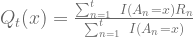
The function I indicates if the action has been chosen at the particular time (it’s an Indicator function) and the function R is the observed reward.
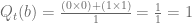
So for action a,

For action b,
Therefore, action a will not be selected by the Greedy Policy, 
 -Greedy Policy
The 
With the probability 
With probability 


So to work out what the probability of selecting action a is, we’ll combine the two probabilities:

Upper Confidence Bounds (UCB) Policy
UCB is an interesting policy that tries to balance the exploration/exploitation trade off via the hyperparamter C. If C is set to 0, then you have a greedy policy. As C increases, you are giving more opportunity to exploration, in other words, selecting alternative actions.

![U_{t}(x)=c~\sqrt[]{\frac{ln(t)}{n_{t}(x)}}](https://s0.wp.com/latex.php?latex=U_%7Bt%7D%28x%29%3Dc%7E%5Csqrt%5B%5D%7B%5Cfrac%7Bln%28t%29%7D%7Bn_%7Bt%7D%28x%29%7D%7D+&bg=ffffff&fg=5e5e5e&s=0&c=20201002)
Both 


![\Rightarrow~argmax_{x \in A} Q_{t}(x)+~c~\sqrt[]{\frac{ln(t)}{1}}](https://s0.wp.com/latex.php?latex=%5CRightarrow%7Eargmax_%7Bx+%5Cin+A%7D+Q_%7Bt%7D%28x%29%2B%7Ec%7E%5Csqrt%5B%5D%7B%5Cfrac%7Bln%28t%29%7D%7B1%7D%7D&bg=ffffff&fg=5e5e5e&s=0&c=20201002)
As before, 
Thompson Sampling
A probability matching policy selects an action based on the probability that it is the best action. Thompson Sampling does this by calculating a probability of the expected reward for each action, and then selecting the action that has the maximum.
This question posed a bit of difficulty. There is an error in the video presentation at time 1:47:50, which caused me a bit of confusion. At that point, the procedure for updating the posterior for the beta distribution Beta(xa,ya) is introduced, but it is incorrect. The posterior updates are swapped around. The correct update should be:

Therfore, the values of 

| Action a | Action b | |
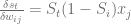
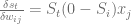
 |  | |
 |  | |
 |  |  |
The values of 


For completion, the expected values of these distributions are:
![\mathbb{E}[x] = \mu = \frac{\alpha}{\alpha + \beta}](https://s0.wp.com/latex.php?latex=%5Cmathbb%7BE%7D%5Bx%5D+%3D+%5Cmu+%3D+%5Cfrac%7B%5Calpha%7D%7B%5Calpha+%2B+%5Cbeta%7D&bg=ffffff&fg=5e5e5e&s=1&c=20201002)
For Action a, this is 1/3 and for Action b, this is 2/3.
Let’s look at the Probability Density Functions for each of the actions. The standard Beta Distribution is given by:
![\frac{1}{B(\alpha,\beta)}[{x}^{\alpha-1}{(1-x)}^{\beta-1}]](https://s0.wp.com/latex.php?latex=%5Cfrac%7B1%7D%7BB%28%5Calpha%2C%5Cbeta%29%7D%5B%7Bx%7D%5E%7B%5Calpha-1%7D%7B%281-x%29%7D%5E%7B%5Cbeta-1%7D%5D&bg=ffffff&fg=5e5e5e&s=1&c=20201002)
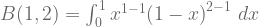
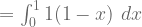
In particular, the beta function itself, “B” (the denominator of the fraction in that equation) is expressed by:

For action “a”, the value of the Beta function is:

![= \large[x-\frac{x^{2}}{2}\large]_{0}^{1}](https://s0.wp.com/latex.php?latex=%3D+%5Clarge%5Bx-%5Cfrac%7Bx%5E%7B2%7D%7D%7B2%7D%5Clarge%5D_%7B0%7D%5E%7B1%7D&bg=ffffff&fg=5e5e5e&s=1&c=20201002)
![= \large[1-\frac{1^{2}}{2}\large]-\large[0-\frac{0^{2}}{2}\large] = \frac{1}{2}](https://s0.wp.com/latex.php?latex=%3D+%5Clarge%5B1-%5Cfrac%7B1%5E%7B2%7D%7D%7B2%7D%5Clarge%5D-%5Clarge%5B0-%5Cfrac%7B0%5E%7B2%7D%7D%7B2%7D%5Clarge%5D+%3D+%5Cfrac%7B1%7D%7B2%7D&bg=ffffff&fg=5e5e5e&s=1&c=20201002)
For action “b”, the value of the Beta function is:


![= \large[\frac{x^{2}}{2}\large]_{0}^{1}](https://s0.wp.com/latex.php?latex=%3D+%5Clarge%5B%5Cfrac%7Bx%5E%7B2%7D%7D%7B2%7D%5Clarge%5D_%7B0%7D%5E%7B1%7D&bg=ffffff&fg=5e5e5e&s=1&c=20201002)
![= \large[\frac{1^{2}}{2}\large] - \large[\frac{0^{2}}{2}\large] = \frac{1}{2}](https://s0.wp.com/latex.php?latex=%3D+%5Clarge%5B%5Cfrac%7B1%5E%7B2%7D%7D%7B2%7D%5Clarge%5D+-+%5Clarge%5B%5Cfrac%7B0%5E%7B2%7D%7D%7B2%7D%5Clarge%5D+%3D+%5Cfrac%7B1%7D%7B2%7D&bg=ffffff&fg=5e5e5e&s=1&c=20201002)
Now we can calculate the Probability Density Functions for both actions:
PDF for action a:


PDF for action b (using y instead of x as the random variable):

The joint PDF for the actions is given by:

Now that we have the joint probability for the actions, we can calculate the probability that the next action selected will be action “a” as follows:

![= \int_{0}^{1} \large(\large[(2-2x)y^{2}\large]_{0}^{x}) ~dx](https://s0.wp.com/latex.php?latex=%3D+%5Cint_%7B0%7D%5E%7B1%7D+%5Clarge%28%5Clarge%5B%282-2x%29y%5E%7B2%7D%5Clarge%5D_%7B0%7D%5E%7Bx%7D%29+%7Edx+&bg=ffffff&fg=5e5e5e&s=1&c=20201002)
![= \int_{0}^{1} \large(\large[(2-2x)x^{2}\large] - \large[(2-2x)0^{2}\large]\large) ~dx](https://s0.wp.com/latex.php?latex=%3D+%5Cint_%7B0%7D%5E%7B1%7D+%5Clarge%28%5Clarge%5B%282-2x%29x%5E%7B2%7D%5Clarge%5D+-+%5Clarge%5B%282-2x%290%5E%7B2%7D%5Clarge%5D%5Clarge%29+%7Edx+&bg=ffffff&fg=5e5e5e&s=1&c=20201002)


![= \large[\frac{2x^{3}}{3} - \frac{2x^{4}}{4}\large]_{0}^{1}](https://s0.wp.com/latex.php?latex=%3D+%5Clarge%5B%5Cfrac%7B2x%5E%7B3%7D%7D%7B3%7D+-+%5Cfrac%7B2x%5E%7B4%7D%7D%7B4%7D%5Clarge%5D_%7B0%7D%5E%7B1%7D+&bg=ffffff&fg=5e5e5e&s=1&c=20201002)
![= \large[\frac{2(1)^{3}}{3} - \frac{2(1)^{4}}{4}\large] - \large[\frac{2(0)^{3}}{3} - \frac{2(0)^{4}}{4}\large]](https://s0.wp.com/latex.php?latex=%3D+%5Clarge%5B%5Cfrac%7B2%281%29%5E%7B3%7D%7D%7B3%7D+-+%5Cfrac%7B2%281%29%5E%7B4%7D%7D%7B4%7D%5Clarge%5D+-+%5Clarge%5B%5Cfrac%7B2%280%29%5E%7B3%7D%7D%7B3%7D+-+%5Cfrac%7B2%280%29%5E%7B4%7D%7D%7B4%7D%5Clarge%5D+&bg=ffffff&fg=5e5e5e&s=1&c=20201002)


So using Thompson Sampling, the probability of selecting action a is:

Note that in the video, the answer is given as 1/4. This is corrected later in the comments.
Conclusion
Hopefully, you found these answers and explanations useful. If so, please let me know in the comments below. Please also let me know if you find any errors and I’ll gladly correct them.


![\frac{\Delta XE}{\Delta S} = \left[ \frac{\delta XE}{\delta S_{1}} \frac{\delta XE}{\delta S_{2}} \ldots \frac{\delta XE}{\delta S_{t}} \right]](https://s0.wp.com/latex.php?latex=%5Cfrac%7B%5CDelta+XE%7D%7B%5CDelta+S%7D+%3D+%5Cleft%5B++%5Cfrac%7B%5Cdelta+XE%7D%7B%5Cdelta+S_%7B1%7D%7D+%5Cfrac%7B%5Cdelta+XE%7D%7B%5Cdelta+S_%7B2%7D%7D+%5Cldots+%5Cfrac%7B%5Cdelta+XE%7D%7B%5Cdelta+S_%7Bt%7D%7D++%5Cright%5D+&bg=ffffff&fg=5e5e5e&s=0&c=20201002)
![\frac{\Delta XE}{\Delta S} = \left[ \ldots \frac{\delta XE}{\delta S_{t}} \ldots \right]](https://s0.wp.com/latex.php?latex=%5Cfrac%7B%5CDelta+XE%7D%7B%5CDelta+S%7D+%3D+%5Cleft%5B+%5Cldots+%5Cfrac%7B%5Cdelta+XE%7D%7B%5Cdelta+S_%7Bt%7D%7D+%5Cldots+%5Cright%5D&bg=ffffff&fg=5e5e5e&s=0&c=20201002)
![\frac{\Delta XE}{\Delta S} = \left[ \ldots \frac{\delta -(Y_{c}\textup{log}(S_{c}))}{\delta S_{c}} \ldots \right]](https://s0.wp.com/latex.php?latex=%5Cfrac%7B%5CDelta+XE%7D%7B%5CDelta+S%7D+%3D+%5Cleft%5B+%5Cldots+%5Cfrac%7B%5Cdelta+-%28Y_%7Bc%7D%5Ctextup%7Blog%7D%28S_%7Bc%7D%29%29%7D%7B%5Cdelta+S_%7Bc%7D%7D+%5Cldots+%5Cright%5D&bg=ffffff&fg=5e5e5e&s=0&c=20201002)
 is 1, so we are left with:
![\frac{\Delta XE}{\Delta S} = \left[ \ldots \frac{\delta -\textup{log}(S_{c})}{\delta S_{c}} \ldots \right]](https://s0.wp.com/latex.php?latex=%5Cfrac%7B%5CDelta+XE%7D%7B%5CDelta+S%7D+%3D+%5Cleft%5B+%5Cldots+%5Cfrac%7B%5Cdelta+-%5Ctextup%7Blog%7D%28S_%7Bc%7D%29%7D%7B%5Cdelta+S_%7Bc%7D%7D+%5Cldots+%5Cright%5D&bg=ffffff&fg=5e5e5e&s=0&c=20201002)
 :
:![\frac{\Delta XE}{\Delta S} = \left[ \ldots -\frac{1}{S_{c}} \ldots \right]](https://s0.wp.com/latex.php?latex=%5Cfrac%7B%5CDelta+XE%7D%7B%5CDelta+S%7D+%3D+%5Cleft%5B+%5Cldots+-%5Cfrac%7B1%7D%7BS_%7Bc%7D%7D+%5Cldots+%5Cright%5D&bg=ffffff&fg=5e5e5e&s=0&c=20201002)

 and in the previous posts, we calculated
  and
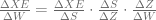
and  . To calculate the overall changes to the weights, we simply carry out a dot product of all those matrices:
 can be calculated using:
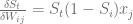


 . So each element in the derivative where i = c becomes:


 j) individual weights in W. Therefore, our matrix of derivatives is going to be of dimensions (K, (i
 ![\frac{\delta{S}}{\delta{x}} = \left [ \begin{array}{ccc} \frac{\delta{z_{1}}}{\delta{w_{11}}} & \ldots & \frac{\delta{z_{1}}} {\delta{w_{53}}} \\ \ldots & \frac{\delta{z_{k}}}{\delta{w_{ij}}} & \ldots \\ \frac{\delta{z_{K}}}{\delta{w_{11}}} & \ldots & \frac{\delta{z_{K}}} {\delta{w_{53}}} \end{array} \right ]](https://s0.wp.com/latex.php?latex=%5Cfrac%7B%5Cdelta%7BS%7D%7D%7B%5Cdelta%7Bx%7D%7D+%3D+%5Cleft+%5B+%5Cbegin%7Barray%7D%7Bccc%7D+%5Cfrac%7B%5Cdelta%7Bz_%7B1%7D%7D%7D%7B%5Cdelta%7Bw_%7B11%7D%7D%7D+%26+%5Cldots+%26+%5Cfrac%7B%5Cdelta%7Bz_%7B1%7D%7D%7D+%7B%5Cdelta%7Bw_%7B53%7D%7D%7D+%5C%5C++%5Cldots+%26+%5Cfrac%7B%5Cdelta%7Bz_%7Bk%7D%7D%7D%7B%5Cdelta%7Bw_%7Bij%7D%7D%7D+%26+%5Cldots+%5C%5C+%5Cfrac%7B%5Cdelta%7Bz_%7BK%7D%7D%7D%7B%5Cdelta%7Bw_%7B11%7D%7D%7D+%26+%5Cldots+%26+%5Cfrac%7B%5Cdelta%7Bz_%7BK%7D%7D%7D+%7B%5Cdelta%7Bw_%7B53%7D%7D%7D+%5Cend%7Barray%7D+%5Cright+%5D&bg=ffffff&fg=5e5e5e&s=0&c=20201002)


 with respect to each of the inputs
  . For example:
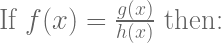
![f'(x)=\frac{g'(x)h(x)-h'(x)g(x)}{[h(x)]^{2}}](https://s0.wp.com/latex.php?latex=f%27%28x%29%3D%5Cfrac%7Bg%27%28x%29h%28x%29-h%27%28x%29g%28x%29%7D%7B%5Bh%28x%29%5D%5E%7B2%7D%7D&bg=ffffff&fg=5e5e5e&s=3&c=20201002)


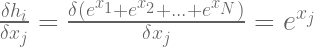
 and where
  :
:![\frac{\delta{\frac{e^{x_{i}}} {\sum_{k=1}^N e^{x_{k}}}}}{\delta{x_{j}}}=\frac{e^{x_{j}}\sum_{k=1}^N e^{x_{k}}-e^{x_{j}}e^{x_{i}}}{\left[\sum_{k=1}^N e^{x_{k}}\right]^{2}}](https://s0.wp.com/latex.php?latex=%5Cfrac%7B%5Cdelta%7B%5Cfrac%7Be%5E%7Bx_%7Bi%7D%7D%7D+%7B%5Csum_%7Bk%3D1%7D%5EN+e%5E%7Bx_%7Bk%7D%7D%7D%7D%7D%7B%5Cdelta%7Bx_%7Bj%7D%7D%7D%3D%5Cfrac%7Be%5E%7Bx_%7Bj%7D%7D%5Csum_%7Bk%3D1%7D%5EN+e%5E%7Bx_%7Bk%7D%7D-e%5E%7Bx_%7Bj%7D%7De%5E%7Bx_%7Bi%7D%7D%7D%7B%5Cleft%5B%5Csum_%7Bk%3D1%7D%5EN+e%5E%7Bx_%7Bk%7D%7D%5Cright%5D%5E%7B2%7D%7D+&bg=ffffff&fg=5e5e5e&s=3&c=20201002)
![\begin{array}{rcl} \frac{\delta{\frac{e^{x_{i}}} {\sum_{k=1}^N e^{x_{k}}}}}{\delta{x_{j}}} & = & \frac{e^{x_{j}}\left(\sum_{k=1}^N e^{x_{k}}-e^{x_{i}}\right)}{\left[\sum_{k=1}^N e^{x_{k}}\right]^{2}}\\ &=&\frac{e^{x_{j}}}{\sum_{k=1}^N e^{x_{k}}} \dot{}\frac{\sum_{k=1}^N e^{x_{k}}-e^{x_{i}}}{\sum_{k=1}^N e^{x_{k}}}\\ &=&\frac{e^{x_{j}}}{\sum_{k=1}^N e^{x_{k}}} \left(\frac{\sum_{k=1}^N e^{x_{k}}}{\sum_{k=1}^N e^{x_{k}}}-\frac{e^{x_{i}}}{\sum_{k=1}^N e^{x_{k}}}\right)\\ &=&\frac{e^{x_{j}}}{\sum_{k=1}^N e^{x_{k}}} \left(1-\frac{e^{x_{i}}}{\sum_{k=1}^N e^{x_{k}}}\right)\\ &=&\sigma(x_{j})(1-\sigma(x_{i})) \end{array}](https://s0.wp.com/latex.php?latex=%5Cbegin%7Barray%7D%7Brcl%7D+%5Cfrac%7B%5Cdelta%7B%5Cfrac%7Be%5E%7Bx_%7Bi%7D%7D%7D+%7B%5Csum_%7Bk%3D1%7D%5EN+e%5E%7Bx_%7Bk%7D%7D%7D%7D%7D%7B%5Cdelta%7Bx_%7Bj%7D%7D%7D+%26+%3D+%26+%5Cfrac%7Be%5E%7Bx_%7Bj%7D%7D%5Cleft%28%5Csum_%7Bk%3D1%7D%5EN+e%5E%7Bx_%7Bk%7D%7D-e%5E%7Bx_%7Bi%7D%7D%5Cright%29%7D%7B%5Cleft%5B%5Csum_%7Bk%3D1%7D%5EN+e%5E%7Bx_%7Bk%7D%7D%5Cright%5D%5E%7B2%7D%7D%5C%5C+%26%3D%26%5Cfrac%7Be%5E%7Bx_%7Bj%7D%7D%7D%7B%5Csum_%7Bk%3D1%7D%5EN+e%5E%7Bx_%7Bk%7D%7D%7D+%5Cdot%7B%7D%5Cfrac%7B%5Csum_%7Bk%3D1%7D%5EN+e%5E%7Bx_%7Bk%7D%7D-e%5E%7Bx_%7Bi%7D%7D%7D%7B%5Csum_%7Bk%3D1%7D%5EN+e%5E%7Bx_%7Bk%7D%7D%7D%5C%5C+%26%3D%26%5Cfrac%7Be%5E%7Bx_%7Bj%7D%7D%7D%7B%5Csum_%7Bk%3D1%7D%5EN+e%5E%7Bx_%7Bk%7D%7D%7D+%5Cleft%28%5Cfrac%7B%5Csum_%7Bk%3D1%7D%5EN+e%5E%7Bx_%7Bk%7D%7D%7D%7B%5Csum_%7Bk%3D1%7D%5EN+e%5E%7Bx_%7Bk%7D%7D%7D-%5Cfrac%7Be%5E%7Bx_%7Bi%7D%7D%7D%7B%5Csum_%7Bk%3D1%7D%5EN+e%5E%7Bx_%7Bk%7D%7D%7D%5Cright%29%5C%5C+%26%3D%26%5Cfrac%7Be%5E%7Bx_%7Bj%7D%7D%7D%7B%5Csum_%7Bk%3D1%7D%5EN+e%5E%7Bx_%7Bk%7D%7D%7D+%5Cleft%281-%5Cfrac%7Be%5E%7Bx_%7Bi%7D%7D%7D%7B%5Csum_%7Bk%3D1%7D%5EN+e%5E%7Bx_%7Bk%7D%7D%7D%5Cright%29%5C%5C+%26%3D%26%5Csigma%28x_%7Bj%7D%29%281-%5Csigma%28x_%7Bi%7D%29%29+%5Cend%7Barray%7D+&bg=ffffff&fg=5e5e5e&s=3&c=20201002)
 :
:![\begin{array}{rcl} \frac{\delta{\frac{e^{x_{i}}} {\sum_{k=1}^N e^{x_{k}}}}}{\delta{x_{j}}}&=&\frac{0-e^{x_{j}}e^{x_{i}}}{\left[\sum_{k=1}^N e^{x_{k}}\right]^{2}}\\ &=&0-\frac{e^{x_{j}}}{\sum_{k=1}^N e^{x_{k}}}\dot{}\frac{e^{x_{i}}}{\sum_{k=1}^N e^{x_{k}}}\\ &=&0-\sigma(x_{j})\sigma(x_{i}) \end{array}](https://s0.wp.com/latex.php?latex=%5Cbegin%7Barray%7D%7Brcl%7D+%5Cfrac%7B%5Cdelta%7B%5Cfrac%7Be%5E%7Bx_%7Bi%7D%7D%7D+%7B%5Csum_%7Bk%3D1%7D%5EN+e%5E%7Bx_%7Bk%7D%7D%7D%7D%7D%7B%5Cdelta%7Bx_%7Bj%7D%7D%7D%26%3D%26%5Cfrac%7B0-e%5E%7Bx_%7Bj%7D%7De%5E%7Bx_%7Bi%7D%7D%7D%7B%5Cleft%5B%5Csum_%7Bk%3D1%7D%5EN+e%5E%7Bx_%7Bk%7D%7D%5Cright%5D%5E%7B2%7D%7D%5C%5C+%26%3D%260-%5Cfrac%7Be%5E%7Bx_%7Bj%7D%7D%7D%7B%5Csum_%7Bk%3D1%7D%5EN+e%5E%7Bx_%7Bk%7D%7D%7D%5Cdot%7B%7D%5Cfrac%7Be%5E%7Bx_%7Bi%7D%7D%7D%7B%5Csum_%7Bk%3D1%7D%5EN+e%5E%7Bx_%7Bk%7D%7D%7D%5C%5C+%26%3D%260-%5Csigma%28x_%7Bj%7D%29%5Csigma%28x_%7Bi%7D%29+%5Cend%7Barray%7D&bg=ffffff&fg=5e5e5e&s=3&c=20201002)


![\frac{\delta{S}}{\delta{x}} = \left [ \begin{array}{ccc} \frac{\delta{S_{1}}}{\delta{x_{1}}} & \ldots & \frac{\delta{S_{1}}}{\delta{x_{N}}} \\ \ldots & \frac{\delta{S_{i}}}{\delta{x_{j}}} & \ldots \\ \frac{\delta{S_{N}}}{\delta{x_{1}}} & \ldots & \frac{\delta{S_{N}}}{\delta{x_{N}}} \end{array} \right ]](https://s0.wp.com/latex.php?latex=%5Cfrac%7B%5Cdelta%7BS%7D%7D%7B%5Cdelta%7Bx%7D%7D+%3D+%5Cleft+%5B+%5Cbegin%7Barray%7D%7Bccc%7D+%5Cfrac%7B%5Cdelta%7BS_%7B1%7D%7D%7D%7B%5Cdelta%7Bx_%7B1%7D%7D%7D+%26+%5Cldots+%26+%5Cfrac%7B%5Cdelta%7BS_%7B1%7D%7D%7D%7B%5Cdelta%7Bx_%7BN%7D%7D%7D+%5C%5C+%5Cldots+%26+%5Cfrac%7B%5Cdelta%7BS_%7Bi%7D%7D%7D%7B%5Cdelta%7Bx_%7Bj%7D%7D%7D+%26+%5Cldots+%5C%5C+%5Cfrac%7B%5Cdelta%7BS_%7BN%7D%7D%7D%7B%5Cdelta%7Bx_%7B1%7D%7D%7D+%26+%5Cldots+%26+%5Cfrac%7B%5Cdelta%7BS_%7BN%7D%7D%7D%7B%5Cdelta%7Bx_%7BN%7D%7D%7D+%5Cend%7Barray%7D+%5Cright+%5D+&bg=ffffff&fg=5e5e5e&s=3&c=20201002)
![\frac{\delta{S}}{\delta{x}} = \left [ \begin{array}{ccc} \sigma(x_{1}) - \sigma(x_{1})\sigma(x_{1}) & \ldots & 0-\sigma(x_{1})\sigma(x_{N}) \\ \ldots & \sigma(x_{j}) - \sigma(x_{j})\sigma(x_{i}) & \ldots \\ 0-\sigma(x_{N})\sigma(x_{1}) & \ldots & \sigma(x_{N}) - \sigma(x_{N})\sigma(x_{N}) \end{array} \right ]](https://s0.wp.com/latex.php?latex=%5Cfrac%7B%5Cdelta%7BS%7D%7D%7B%5Cdelta%7Bx%7D%7D+%3D+%5Cleft+%5B+%5Cbegin%7Barray%7D%7Bccc%7D+%5Csigma%28x_%7B1%7D%29+-+%5Csigma%28x_%7B1%7D%29%5Csigma%28x_%7B1%7D%29+%26+%5Cldots+%26+0-%5Csigma%28x_%7B1%7D%29%5Csigma%28x_%7BN%7D%29+%5C%5C+%5Cldots+%26+%5Csigma%28x_%7Bj%7D%29+-+%5Csigma%28x_%7Bj%7D%29%5Csigma%28x_%7Bi%7D%29+%26+%5Cldots+%5C%5C+0-%5Csigma%28x_%7BN%7D%29%5Csigma%28x_%7B1%7D%29+%26+%5Cldots+%26+%5Csigma%28x_%7BN%7D%29+-+%5Csigma%28x_%7BN%7D%29%5Csigma%28x_%7BN%7D%29+%5Cend%7Barray%7D+%5Cright+%5D+&bg=ffffff&fg=5e5e5e&s=3&c=20201002)
![\frac{\delta{S}}{\delta{x}} = \left [ \begin{array}{ccc} \sigma(x_{1}) & \ldots & 0 \\ \ldots & \sigma(x_{j}) & \ldots \\ 0 & \ldots & \sigma(x_{N})\end{array} \right ] - \left[ \begin{array}{ccc} \sigma(x_{1})\sigma(x_{1}) & \ldots & \sigma(x_{1})\sigma(x_{N}) \\ \ldots & \sigma(x_{j})\sigma(x_{i}) & \ldots \\ \sigma(x_{N})\sigma(x_{1}) & \ldots & \sigma(x_{N})\sigma(x_{N}) \end{array} \right ]](https://s0.wp.com/latex.php?latex=%5Cfrac%7B%5Cdelta%7BS%7D%7D%7B%5Cdelta%7Bx%7D%7D+%3D+%5Cleft+%5B+%5Cbegin%7Barray%7D%7Bccc%7D+%5Csigma%28x_%7B1%7D%29+%26+%5Cldots+%26+0+%5C%5C+%5Cldots+%26+%5Csigma%28x_%7Bj%7D%29+%26+%5Cldots+%5C%5C+0+%26+%5Cldots+%26+%5Csigma%28x_%7BN%7D%29%5Cend%7Barray%7D+%5Cright+%5D+-+%5Cleft%5B+%5Cbegin%7Barray%7D%7Bccc%7D+%5Csigma%28x_%7B1%7D%29%5Csigma%28x_%7B1%7D%29+%26+%5Cldots+%26+%5Csigma%28x_%7B1%7D%29%5Csigma%28x_%7BN%7D%29+%5C%5C+%5Cldots+%26+%5Csigma%28x_%7Bj%7D%29%5Csigma%28x_%7Bi%7D%29+%26+%5Cldots+%5C%5C+%5Csigma%28x_%7BN%7D%29%5Csigma%28x_%7B1%7D%29+%26+%5Cldots+%26+%5Csigma%28x_%7BN%7D%29%5Csigma%28x_%7BN%7D%29+%5Cend%7Barray%7D+%5Cright+%5D+&bg=ffffff&fg=5e5e5e&s=3&c=20201002)


